MAFFT Background
MAFFT gets its name from its use of Fast Fourier Transform to quickly identify some of the more obvious regions of homology. After identifying these regions, slower dynamic programming approaches are used to join these segments into a full alignment. Thus, the main advantage of the initial version of MAFFT was speed. The speed of MAFFT has made it a favorite method for many phylogenomic studies and it has some alignment algorithms that are very useful for some common data types (e.g. UCEs, hybrid enrichment/capture-seq, RADseq).
MAFFT also uses a transformation of scoring matrices (fully described in the “Scoring system” section on pages 3061 and 3062 of Katoh et al. 2002 so that all of the pairwise scores are positive and costs of multi-position gaps can be computed quickly.
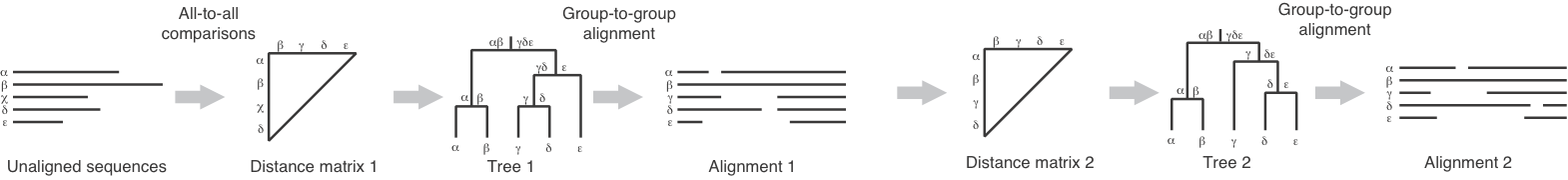
The steps in a MAFFT run are:
- calculation of a crude pairwise distance matrix based shared 6-tuples
- construction of a UPGMA (Unweighted Pair Group Method with Arithmetic Mean) guide tree
- FFT and dynamic programming used in progressive alignment with this initial guide tree
- improved pairwise distance matrix inferred from the alignment of step 3
- improved guide tree constructed from the new distances that were computed in step 4
- repeat of the progressive alignment algorithm (like step 3, but with the new guide tree).
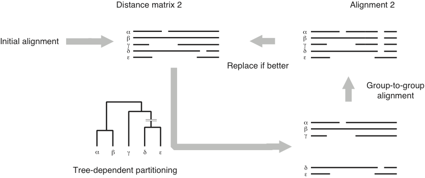
- Then MAFFT repeats the following:
- break the alignment in 2 groups based on the tree
- realign these groups
- accept this alignment if it improves the score.
The first 3 steps are called FFT-NS-1. Continuing through step 6 is called FFT-NS-2. And including the iterative improvements is referred to as FFT-NS-2-i.
The following figure (from the nice review by Katoh and Toh (2008)) diagrams FFT-NS-2:
The iterative improvement steps mentioned in step 7 (which are used if you use the FFT-NS-2-i version of the algorithm) are depicted as:
Katoh et al. 2005 added consistency-based scoring in the iterative refinement stage. G-INS-i uses global alignments to construct the library of pairwise alignments used to assess consistency. L-INS-i uses local pairwise alignments with affine gaps to form the library, and E-INS-i uses local alignments with a generalized affine gap cost (which allows for an unalignable cost in addition to gap opening and gap extension costs). The contexts in which you would want to use each of these algorithms is shown below (from Figure 3 of Katoh and Toh (2008)). X’s in the figure represent aligned residues and o’s represent unalignable residues:
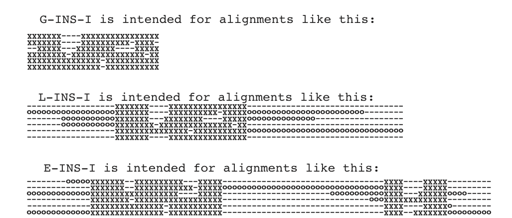
We do encounter such cases in real biological datasets. For example L-INS-I is useful for hybrid enrichment (Breinholt et al. 2018) or UCES (Faircloth 2016).
References
Breinholt JW, Earl C, Lemmon AR, Lemmon EM, Xiao L, Kawahara AY. 2017. Resolving relationships among the megadiverse butterflies and moths with a novel pipeline for anchored phylogenomics. Syst Biol. 67:78-93.
Faircloth BC. 2016. PHYLUCE is a software package for the analysis of conserved genomic loci. Bioinformatics. 32:786-788.
Katoh K, Misawa K, Kuma K, Miyata T. 2002. MAFFT: a novel method for rapid multiple sequence alignment based on fast Fourier transform. Nucleic Acids Res. 30:3059-3066.
Katoh K, Kuma K, Toh H, Miyata T. 2005. MAFFT version 5: improvement in accuracy of multiple sequence alignment. Nucleic Acids Res. 33:511-518.
Katoh K, Toh H. 2008. Recent developments in the MAFFT multiple sequence alignment program. Brief Bioinform. 9:286-298.